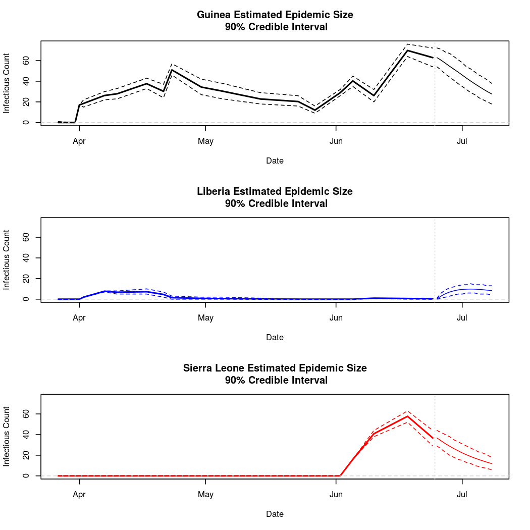
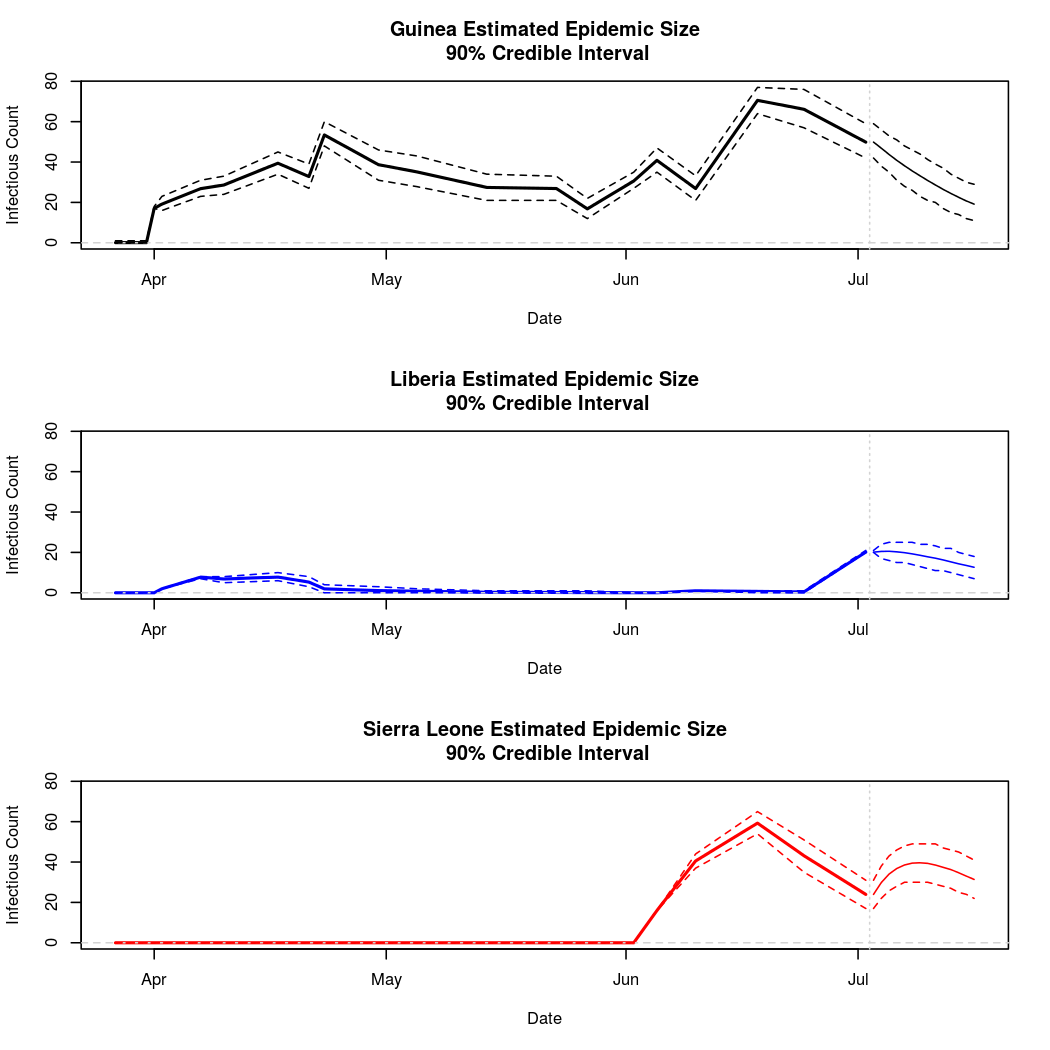
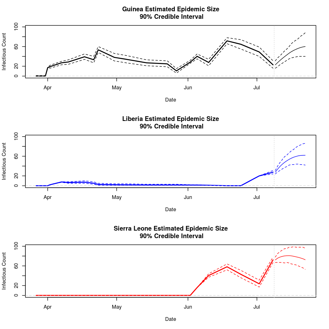
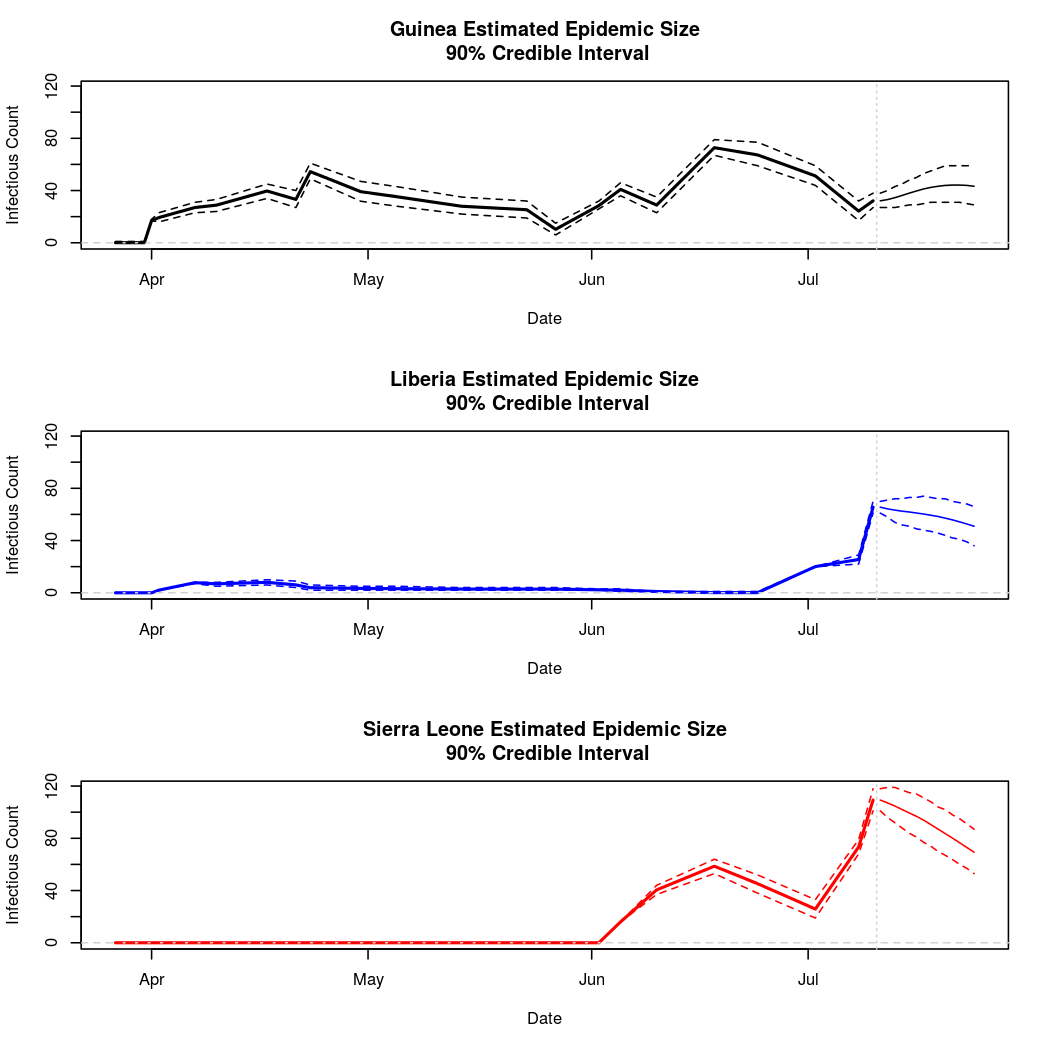
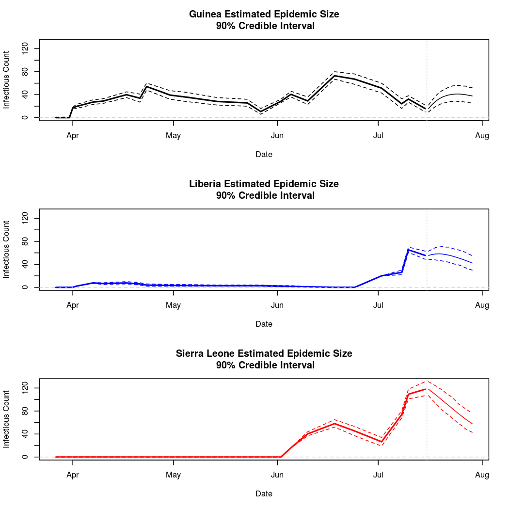
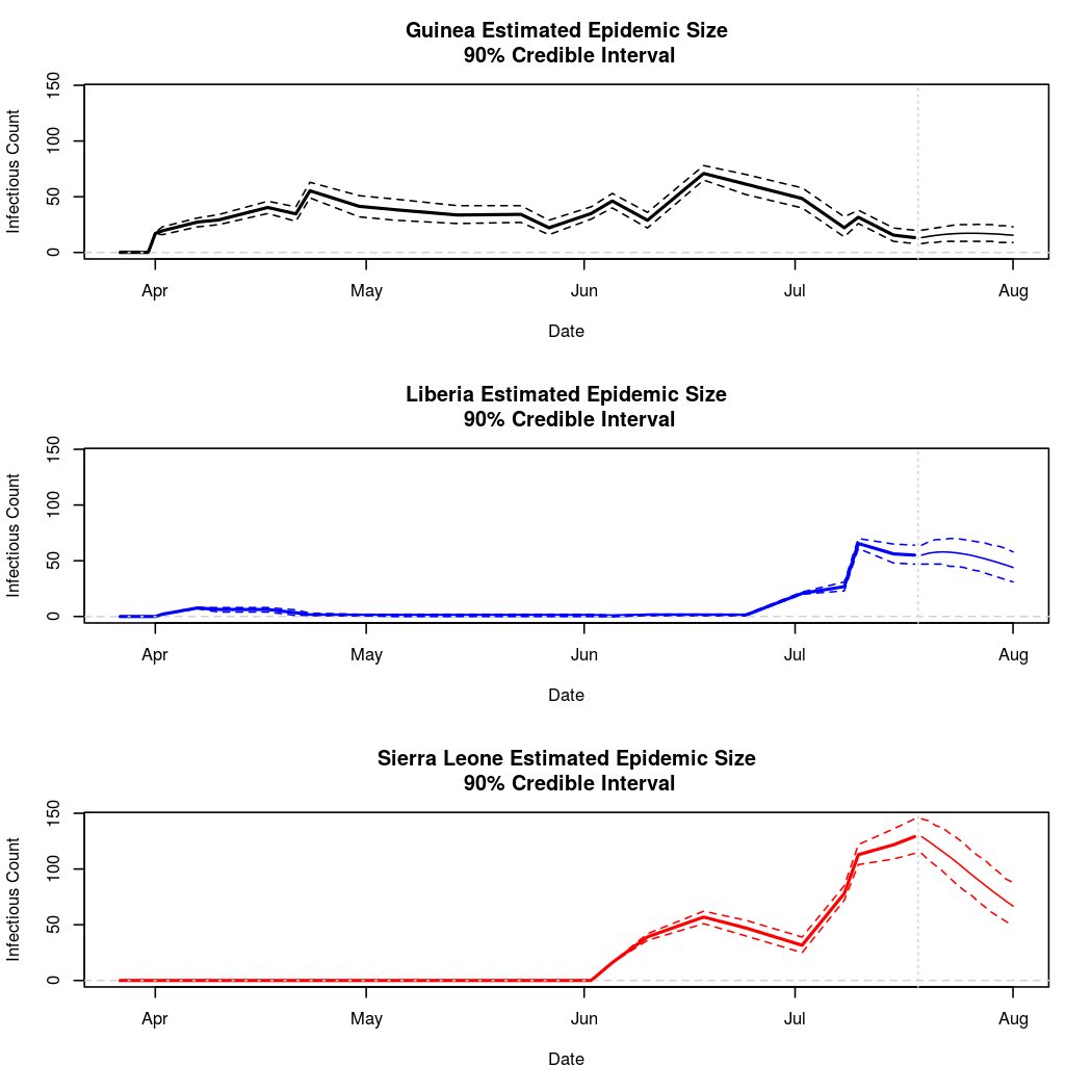
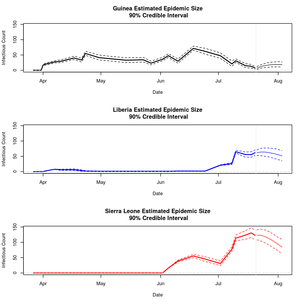
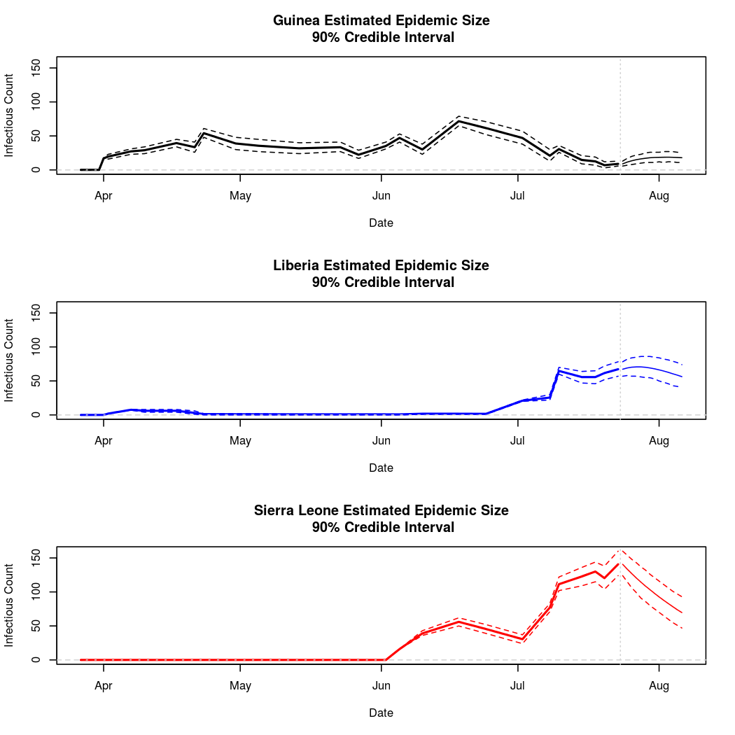
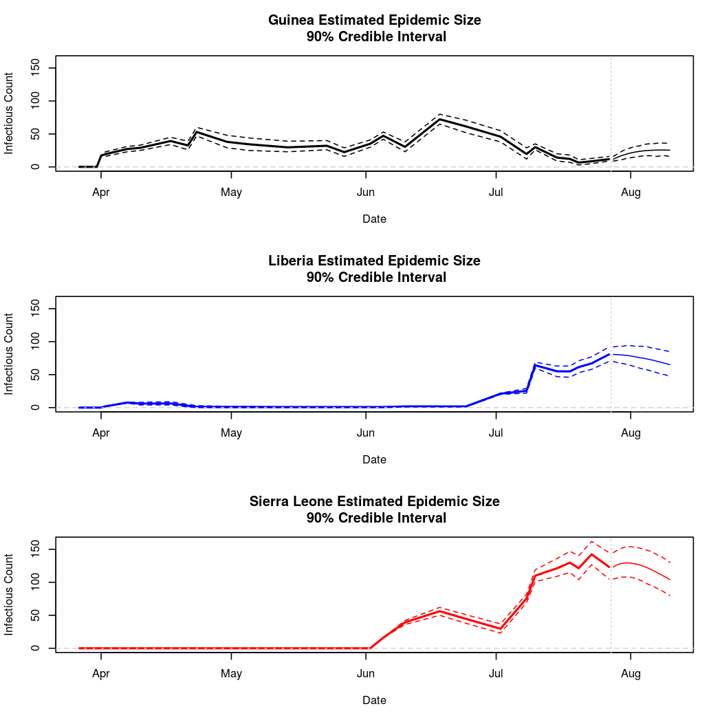
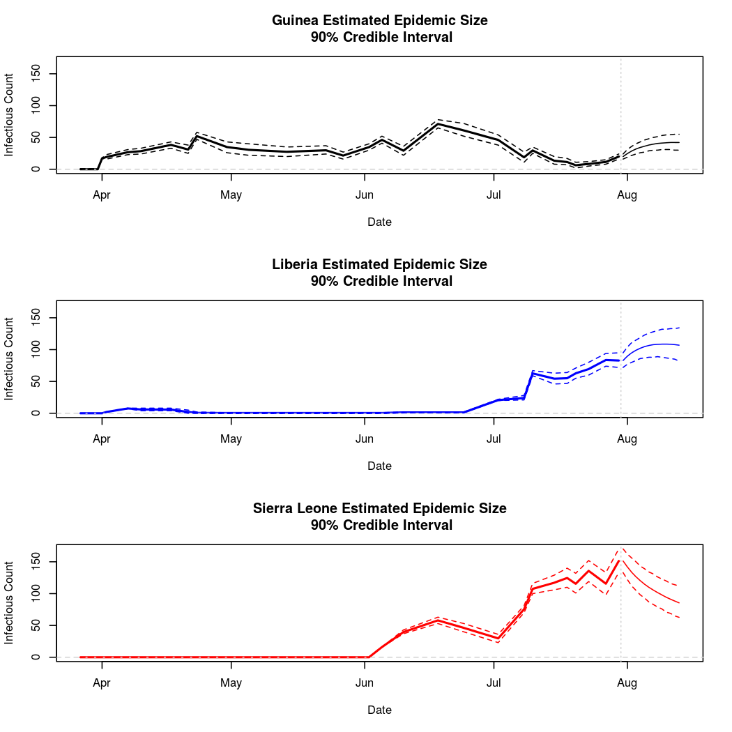
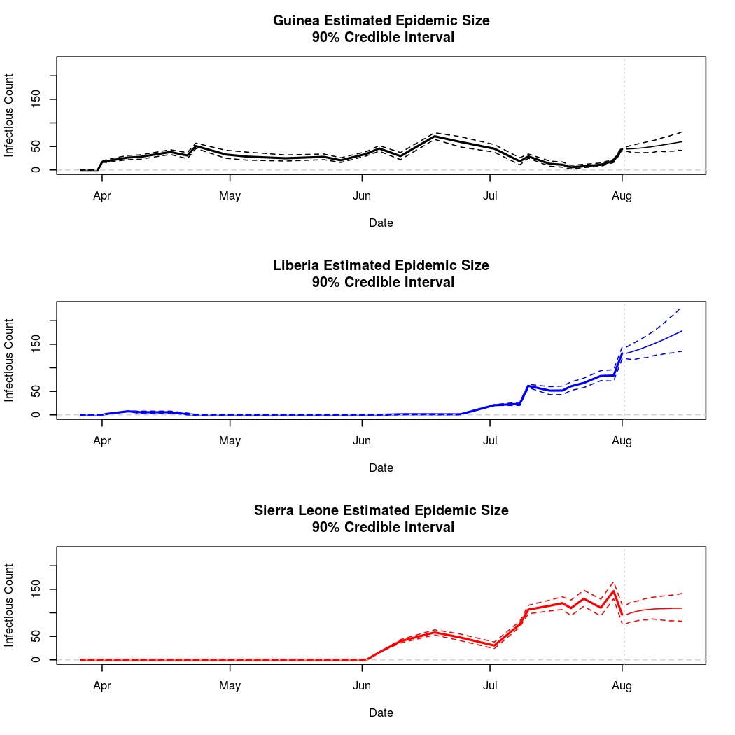
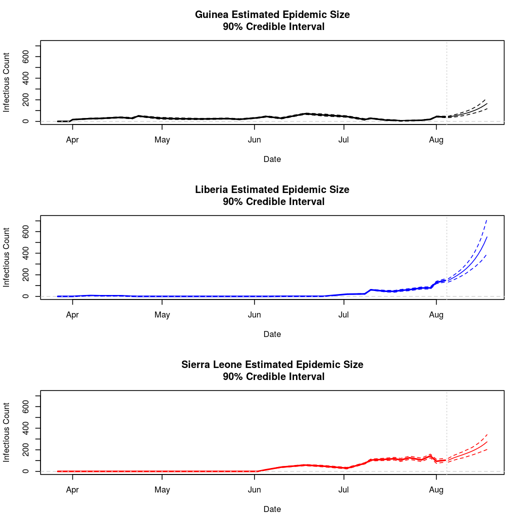
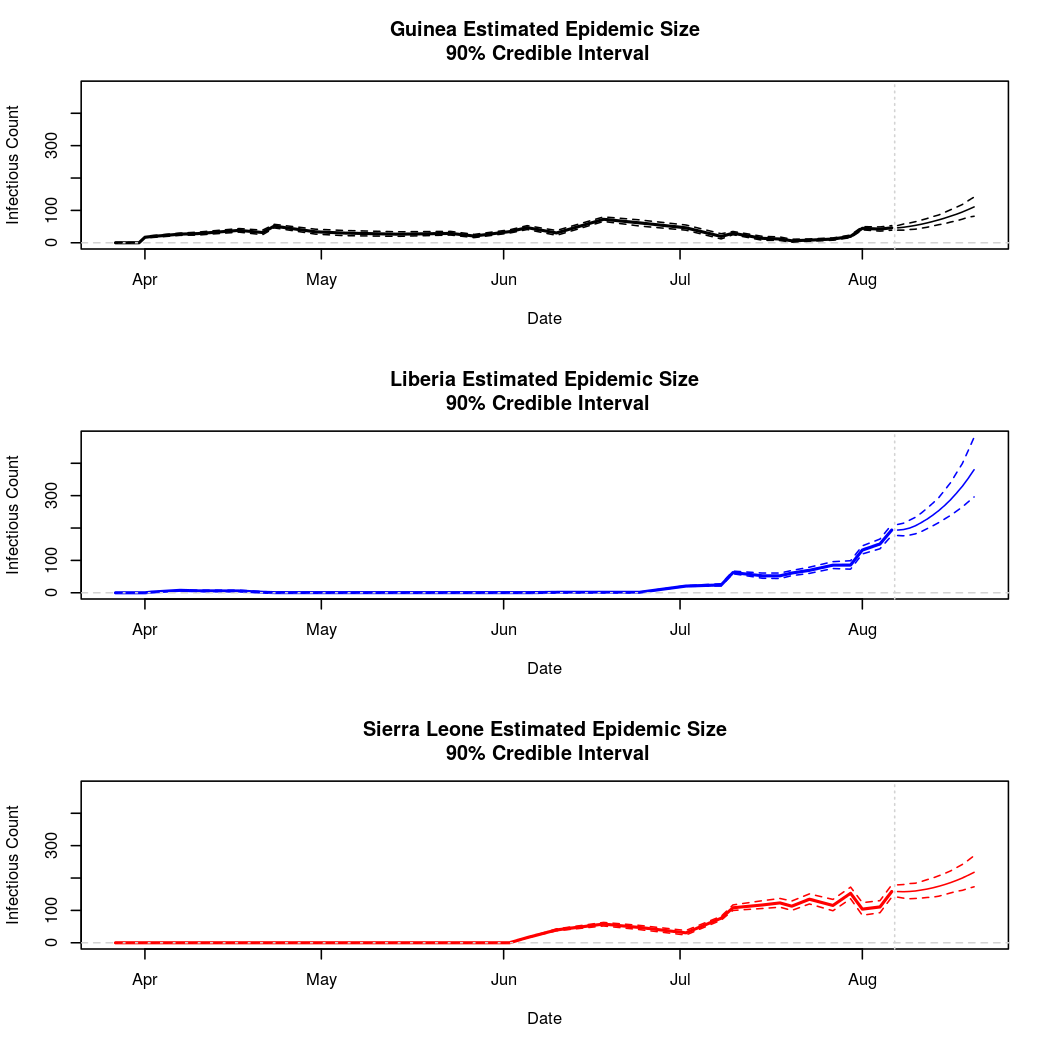
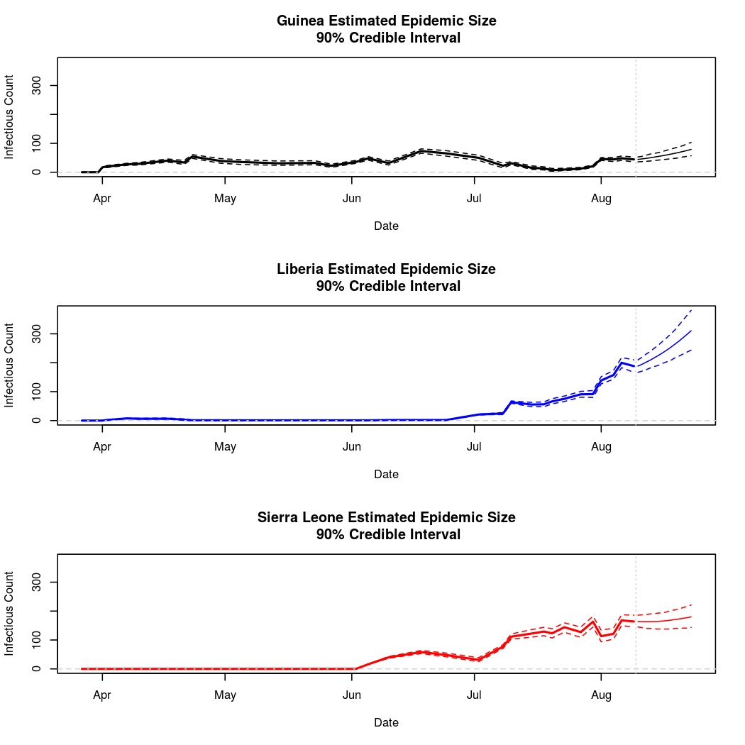
The following chart tracks the prediction performance of the cubic spline SEIR model over the course of the epidemic so far. Prediction windows are two weeks in length. These predictions are based on single MCMC chains, as convergence behavior for this model/data was assessed in the initial analysis linked above.
library(coda) # Load the coda library for MCMC convergence diagnosis
## Loading required package: lattice
library(spatialSEIR) # Load the spatialSEIR library to perform the modeling.
## Loading required package: Rcpp
library(XML) # Load the XML library to read in data from Wikipedia
library(splines) # Load the splines library to build the temporal basis.


############################################
## Define Document Compilation Parameters ##
############################################

documentCompilationMode = "release"
#documentCompilationMode = "debug"

numConvergenceBatches = ifelse(documentCompilationMode == "release", 250, 50)
convergenceBatchSize =  ifelse(documentCompilationMode == "release", 10000, 100)

url = 'http://en.wikipedia.org/wiki/2014_West_Africa_Ebola_outbreak'
tbls = readHTMLTable(url)
dat = tbls[[2]] # This line changes depending on the page formatting.

rptDate = as.Date(dat[2:nrow(dat),1], "%d %b %Y")
original.rptDate = rptDate
ascendingOrder = order(rptDate)
rptDate = rptDate[ascendingOrder][2:length(rptDate)]
original.rptDate = original.rptDate[ascendingOrder]
Guinea = as.numeric(as.character(dat$V4[2:nrow(dat)]))[ascendingOrder]
Guinea = ifelse(is.na(Guinea), 0, Guinea)
Liberia = as.numeric(as.character(dat$V6[2:nrow(dat)]))[ascendingOrder]
Liberia = ifelse(is.na(Liberia), 0, Liberia)
Sierra.Leone = as.numeric(as.character(dat$V8[2:nrow(dat)]))[ascendingOrder]
Sierra.Leone = ifelse(is.na(Sierra.Leone), 0,Sierra.Leone)

uncumulate = function(x)
{
    out = c(x[2:length(x)]-x[1:(length(x)-1)])
    ifelse(out >= 0, out, 0)
}

makePrediction = function(maxIdx, seedVal=123123)
{
  # Define the data matrix.
  I_star = cbind(uncumulate(Guinea[1:maxIdx]),
                 uncumulate(Liberia[1:maxIdx]),
                 uncumulate(Sierra.Leone[1:maxIdx]))

  # Define the temporal offset vector to be the number of days reflected in each
  # aggregated record (time between reports).
  offsets = uncumulate(original.rptDate[1:maxIdx])
  rptDate_sub = rptDate[2:maxIdx]

  # Define the simple "distance" matrix. There are 3 countries, all of which
  # share borders. Therefore we simply define a 3x3 matrix with zero diagonals
  # and 0.5 for the off diagonal values. 0.5 is used instead of 1 because
  # this normalized choice makes the matrix row stochastic, which makes the gods
  # of proper posterior distributions happy.
  DM = 0.5*(1-diag(3))

  # Define population sizes for the three countries of interest. This data also
  # from Wikipedia.

  # Guinea, Liberia, Sierra Leone
  N = matrix(c(10057975, 4128572, 6190280), nrow = nrow(I_star),ncol = 3,
             byrow=TRUE)

  # Currently, the fixed and time varying co-variates driving the exposure
  # process must be specified separately This saves computer memory, but
  # makes things a bit more complicated. I might change this at some point.

  # For the fixed covariates, just fit a separate intercept for each location.
  X = diag(3)

  # For the time varying covariates, we first need to define a temporal index
  daysSinceJan = as.numeric(rptDate_sub - as.Date("2014-01-01"))
  daysSinceJan_whole = as.numeric(rptDate - as.Date("2014-01-01"))

  daysSinceJan.predict = ((max(daysSinceJan)+1):(max(daysSinceJan)+60))[1:14]

  splineBasis = ns(daysSinceJan, df = 3)
  splineBasis.predict = predict(splineBasis, daysSinceJan.predict)

  # Guinea, Liberia, Sierra Leone
  N = matrix(c(10057975, 4128572, 6190280), nrow = nrow(I_star),ncol = 3,
             byrow=TRUE)

  X.predict = cbind(diag(3))
  Z = splineBasis
  Z.predict = splineBasis.predict

  # These co-variates are the same for each spatial location,
  # so duplicate them row-wise.
  Z = Z[rep(1:nrow(Z), nrow(X)),]
  Z.predict = Z.predict[rep(1:nrow(Z.predict), nrow(X)),]

  # For convenience, let's combine X and Z for prediction.
  X.pred = cbind(X.predict[rep(1:nrow(X.predict),
                               each = nrow(Z.predict)/nrow(X)),], Z.predict)
  # Define prediction offsets.
  offset.pred = uncumulate(c(daysSinceJan[length(daysSinceJan)], daysSinceJan.predict))

  # There's no reinfection process for Ebola, but we still need to provide dummy
  # values for the reinfection terms. This will be changed (along with most of
  # the R level API) Dummy covariate matrix:
  X_p_rs = matrix(0)
  # Dummy covariate matrix dimension. Why, exactly, am I not just grabbing this
  # kind of thing from Rcpp? No good reason at all: this will be fixed.
  xPrsDim = dim(X_p_rs)
  # Dummy value for reinfection params
  beta_p_rs = rep(0, ncol(X_p_rs))
  # Dummy value for reinfection params prior precision
  betaPrsPriorPrecision = 0.5

  # Get object dimensions. Again, this will be done automatically in the future
  compMatDim = dim(I_star)
  xDim = dim(X)
  zDim = dim(Z)

  # Declare prior parameters for the E to I and I to R probabilities.
  priorAlpha_gammaEI = 250;
  priorBeta_gammaEI = 1000;
  priorAlpha_gammaIR = 140;
  priorBeta_gammaIR = 1000;

  # Declare prior precision for exposure model paramters
  betaPriorPrecision = 0.1

  # Set the reinfection mode to 3, which indicates that S_star, or the newly
  # susceptibles, must remain zero. People are very unlikely to get ebola twice.
  # How were you to know that "3" denotes a traditional SEIR model as opposed to
  # a serial SEIR or SEIRS model? No good reason at all, actually. The planned R
  # API will make the distinction between SEIRmodel SEIRSmodel and
  # SerialSEIRmodel objects, so in the future you won't have to worry about this
  # unless you're digging into the c++ code.
  reinfectionMode = 3

  # steadyStateConstraintPrecision is a loose constraint on net flows
  # between compartments. Setting it to a negative value eliminates
  # the constraint, but it can help with identifiability in cases where
  # there should be a long term equilibrium (endemic disease, for example).
  # We do not need this parameter here.
  steadyStateConstraintPrecision = -1

  # iterationStride determines the delay between saving samples to the specified
  # output file As you can probably tell based on the high number chosen,
  # autocorrelation is currently a big problem for this library
  iterationStride = 1000

  # We don't need no verbose or debug level output
  verbose = FALSE
  debug = FALSE

  # Declare initial tuning parameters for MCMC sampling
  mcmcTuningParams = c(1, # S_star
                       1, # E_star
                       1,  # R_star
                       1,  # S_0
                       1,  # I_0
                       0.05,  # beta
                       0.0,  # beta_p_rs, fixed in this case
                       0.01, # rho
                       0.01, # gamma_ei
                       0.01) # gamma_ir


  # We don't want to re-scale the distance matrix.
  scaleDistanceMode = 0

    # Declare a function which can come up with several different starting values
    # for the model parameters. This will allow us to assess convergence.
    proposeParameters = function(seedVal, chainNumber)
    {
        set.seed(seedVal)
        # 2 to 21 day incubation period according to who
        p_ei = 0.25 + rnorm(1, 0, 0.02)
        # Up to 7 weeks even after recovery
        p_ir = 0.14 + rnorm(1, 0, 0.01)
        gamma_ei=-log(1-p_ei)
        gamma_ir=-log(1-p_ir)

        # Starting value for exposure regression parameters
        beta = rep(0, ncol(X) + ncol(Z))
        beta[1] = 2.5 + rnorm(1,0,0.5)

        rho = 0.1 + rnorm(1,0,0.01) # spatial dependence parameter

        outFileName = paste("./chain_output_ebola_", chainNumber ,".txt", sep = "")

        # Make a crude guess as to the true compartments:
        # S_star, E_star, R_star, and thus S,E,I and R
        proposal = generateCompartmentProposal(I_star, N,
                                               S0 = N[1,]-I_star[1,] - c(86,0,0),
                                               I0 = c(86,0,0),
                                               p_ir = 0.5,
                                               p_rs = 0.00)

        return(list(S0=proposal$S0,
                    E0=proposal$E0,
                    I0=proposal$I0,
                    R0=proposal$R0,
                    S_star=proposal$S_star,
                    E_star=proposal$E_star,
                    I_star=proposal$I_star,
                    R_star=proposal$R_star,
                    rho=rho,
                    beta=beta,
                    gamma_ei=gamma_ei,
                    gamma_ir=gamma_ir,
                    outFileName=outFileName))
  }

  # Make a helper function to run each chain, as well as update the metropolis
  # tuning parameters.
  runSimulation = function(modelObject,
                           numBatches=500,
                           batchSize=20,
                           targetAcceptanceRatio=0.2,
                           tolerance=0.05,
                           proportionChange = 0.1
                          )
  {
      for (batch in 1:numBatches)
      {
          modelObject$simulate(batchSize)
          modelObject$updateSamplingParameters(targetAcceptanceRatio,
                                               tolerance,
                                               proportionChange)
      }
  }

  predictEpidemic = function(beta.pred,
                               X.pred,
                               gamma.ei,
                               gamma.ir,
                               S0,
                               E0,
                               I0,
                               R0,
                               rho,
                               offsets.pred)
    {
        N = (S0+E0+I0+R0)
        p_se_components = matrix(exp(X.pred %*% beta.pred), ncol=length(S0))
        p_se = matrix(0, ncol = length(S0), nrow = nrow(p_se_components))
        p_ei = 1-exp(-gamma.ei*offsets.pred)
        p_ir = 1-exp(-gamma.ir*offsets.pred)
        S_star = matrix(0, ncol=length(S0),nrow = nrow(p_se_components))
        E_star = matrix(0, ncol=length(S0),nrow = nrow(p_se_components))
        I_star = matrix(0, ncol=length(S0),nrow = nrow(p_se_components))
        R_star = matrix(0, ncol=length(S0),nrow = nrow(p_se_components))
        S = matrix(0, ncol=length(S0),nrow = nrow(p_se_components))
        E = matrix(0, ncol=length(S0),nrow = nrow(p_se_components))
        I = matrix(0, ncol=length(S0),nrow = nrow(p_se_components))
        R = matrix(0, ncol=length(S0),nrow = nrow(p_se_components))
        S[1,] = S0
        E[1,] = E0
        I[1,] = I0
        R[1,] = R0
        S_star[1,] = rbinom(rep(1, length(S0)), R0, 0)
        p_se[1,] = 1-exp(-offsets.pred[1]*(I[1,]/N*p_se_components[1,] +
                              rho*(DM %*% (I[1,]/N*p_se_components[1,]))))
        E_star[1,] = rbinom(rep(1, length(S0)), S0, p_se[1,])
        I_star[1,] = rbinom(rep(1, length(S0)), E0, p_ei[1])
        R_star[1,] = rbinom(rep(1, length(S0)), I0, p_ir[1])

        for (i in 2:nrow(S))
        {

          S[i,] = S[i-1,] + S_star[i-1,] - E_star[i-1,]
          E[i,] = E[i-1,] + E_star[i-1,] - I_star[i-1,]
          I[i,] = I[i-1,] + I_star[i-1,] - R_star[i-1,]
          R[i,] = R[i-1,] + R_star[i-1,] - S_star[i-1,]

          p_se[i,] = 1-exp(-offsets.pred[i]*(I[i,]/N*p_se_components[i,] +
                              rho*(DM %*% (I[i,]/N*p_se_components[i,]))))
          S_star[i,] = rbinom(rep(1, length(S0)), R[i,], 0)
          E_star[i,] = rbinom(rep(1, length(S0)), S[i,], p_se[i,])
          I_star[i,] = rbinom(rep(1, length(S0)), E[i,], p_ei[i])
          R_star[i,] = rbinom(rep(1, length(S0)), I[i,], p_ir[i])
        }
        return(list(S=S,E=E,I=I,R=R,
                    S_star=S_star,E_star=E_star,
                    I_star=I_star,R_star=R_star,
                    p_se=p_se,p_ei=p_ei,p_ir=p_ir))
    }

  predict.i = function(i,chainFile,maxIdx)
  {
    dataRow = chainFile[i,]
    rho = dataRow$rho
    beta = c(dataRow$BetaP_SE_0,
             dataRow$BetaP_SE_1,
             dataRow$BetaP_SE_2,
             dataRow$BetaP_SE_3,
             dataRow$BetaP_SE_4,
             dataRow$BetaP_SE_5)

    S0 = c(dataRow[[paste("S_0_", maxIdx-2, sep = "")]],
           dataRow[[paste("S_1_", maxIdx-2, sep = "")]],
           dataRow[[paste("S_2_", maxIdx-2, sep = "")]])
    E0 = c(dataRow[[paste("E_0_", maxIdx-2, sep = "")]],
           dataRow[[paste("E_1_", maxIdx-2, sep = "")]],
           dataRow[[paste("E_2_", maxIdx-2, sep = "")]])
    I0 = c(dataRow[[paste("I_0_", maxIdx-2, sep = "")]],
           dataRow[[paste("I_1_", maxIdx-2, sep = "")]],
           dataRow[[paste("I_2_", maxIdx-2, sep = "")]])
    R0 = c(dataRow[[paste("R_0_", maxIdx-2, sep = "")]],
           dataRow[[paste("R_1_", maxIdx-2, sep = "")]],
           dataRow[[paste("R_2_", maxIdx-2, sep = "")]])

    return(predictEpidemic(beta,
                           X.pred,
                           dataRow$gamma_ei,
                           dataRow$gamma_ir,
                           S0,
                           E0,
                           I0,
                           R0,
                           rho,
                           offset.pred
                           ))
  }

  # Make model object
  proposal = proposeParameters(seedVal, maxIdx)
  SEIRmodel.spline = spatialSEIRModel(compMatDim,
                      xDim,
                      zDim,
                      xPrsDim,
                      proposal$S0,
                      proposal$E0,
                      proposal$I0,
                      proposal$R0,
                      proposal$S_star,
                      proposal$E_star,
                      proposal$I_star,
                      proposal$R_star,
                      offsets,
                      X,
                      Z,
                      X_p_rs,
                      DM,
                      proposal$rho,
                      priorAlpha_gammaEI,
                      priorBeta_gammaEI,
                      priorAlpha_gammaIR,
                      priorBeta_gammaIR,
                      proposal$beta,
                      betaPriorPrecision,
                      beta_p_rs,
                      betaPrsPriorPrecision,
                      proposal$gamma_ei,
                      proposal$gamma_ir,
                      N,
                      proposal$outFileName,
                      iterationStride,
                      steadyStateConstraintPrecision,
                      verbose,
                      debug,
                      mcmcTuningParams,
                      reinfectionMode,
                      scaleDistanceMode)
  SEIRmodel.spline$setRandomSeed(seedVal)
  SEIRmodel.spline$setTrace(0) #Guinea
  SEIRmodel.spline$setTrace(1) #Liberia
  SEIRmodel.spline$setTrace(2) #Sierra Leone

  runSimulation(SEIRmodel.spline)
  SEIRmodel.spline$simulate(1000)
  tm = system.time(runSimulation(SEIRmodel.spline,
                  numBatches=numConvergenceBatches,
                  batchSize=convergenceBatchSize,
                  targetAcceptanceRatio=0.2,
                  tolerance=0.025,
                  proportionChange = 0.05))
  cat(paste("Time elapsed for convergence run: ", round(tm[3]/60,3), " minutes\n", sep = ""))

  chain = read.csv(paste("chain_output_ebola_", maxIdx, ".txt", sep = ""))
  c1 = chain[floor(nrow(chain)/2):nrow(chain),c(1:6,8:10)]


  # Guinea, Liberia, Sierra Leone
  getMeanAndCI = function(loc,tpt,baseStr="I_")
  {
      vec = chain[[paste(baseStr, loc, "_", tpt, sep = "")]]
      vec = vec[floor(length(vec)/2):length(vec)]
      return(c(mean(vec), quantile(vec, probs = c(0.05, 0.95))))
  }

  Guinea.I.Est = sapply(0:(nrow(I_star)- 1), getMeanAndCI, loc=0)
  Liberia.I.Est = sapply(0:(nrow(I_star)- 1), getMeanAndCI, loc=1)
  SierraLeone.I.Est = sapply(0:(nrow(I_star)- 1), getMeanAndCI, loc=2)

  preds = lapply((nrow(chain) - floor(nrow(chain)/2)):
                    nrow(chain), predict.i, maxIdx = maxIdx, chainFile=chain)


  Guinea.Pred = preds[[1]]$I[,1]
  Liberia.Pred = preds[[1]]$I[,2]
  SierraLeone.Pred = preds[[1]]$I[,3]

  for (predIdx in 2:length(preds))
  {
     Guinea.Pred = rbind(Guinea.Pred, preds[[predIdx]]$I[,1])
     Liberia.Pred = rbind(Liberia.Pred, preds[[predIdx]]$I[,2])
     SierraLeone.Pred = rbind(SierraLeone.Pred, preds[[predIdx]]$I[,3])
  }

  Guinea.mean = apply(Guinea.Pred, 2, mean)
  Liberia.mean = apply(Liberia.Pred, 2, mean)
  SierraLeone.mean = apply(SierraLeone.Pred, 2, mean)

  Guinea.LB = apply(Guinea.Pred, 2, quantile, probs = c(0.05))
  Guinea.UB = apply(Guinea.Pred, 2, quantile, probs = c(0.95))

  Liberia.LB = apply(Liberia.Pred, 2, quantile, probs = c(0.05))
  Liberia.UB = apply(Liberia.Pred, 2, quantile, probs = c(0.95))

  SierraLeone.LB = apply(SierraLeone.Pred, 2, quantile, probs = c(0.05))
  SierraLeone.UB = apply(SierraLeone.Pred, 2, quantile, probs = c(0.95))


  return(list("Dates" = list("Est"=daysSinceJan + as.Date("2014-01-01"), "Pred" = daysSinceJan.predict + as.Date("2014-01-01")),
              "Data" = list("Guinea" = list("Est" = Guinea.I.Est, "Pred" = cbind(Guinea.mean, Guinea.LB, Guinea.UB)),
              "Liberia" = list("Est" = Liberia.I.Est, "Pred" = cbind(Liberia.mean, Liberia.LB, Liberia.UB)),
              "SierraLeone" = list("Est" = SierraLeone.I.Est, "Pred" = cbind(SierraLeone.mean, SierraLeone.LB, SierraLeone.UB))),
            "maxIdx" = maxIdx))

}


maxIdxList = lapply(20:33, makePrediction)
## Building Model.
##    Number of Locations: 3
##    Number of Time Points: 19
## Setting index length to be: 14
## Time elapsed for convergence run: 16.622 minutes
## Building Model.
##    Number of Locations: 3
##    Number of Time Points: 20
## Setting index length to be: 15
## Time elapsed for convergence run: 11.481 minutes
## Building Model.
##    Number of Locations: 3
##    Number of Time Points: 21
## Setting index length to be: 15
## Time elapsed for convergence run: 11.13 minutes
## Building Model.
##    Number of Locations: 3
##    Number of Time Points: 22
## Setting index length to be: 16
## Time elapsed for convergence run: 15.996 minutes
## Building Model.
##    Number of Locations: 3
##    Number of Time Points: 23
## Setting index length to be: 17
## Time elapsed for convergence run: 13.942 minutes
## Building Model.
##    Number of Locations: 3
##    Number of Time Points: 24
## Setting index length to be: 18
## Time elapsed for convergence run: 16.472 minutes
## Building Model.
##    Number of Locations: 3
##    Number of Time Points: 25
## Setting index length to be: 18
## Time elapsed for convergence run: 18.7 minutes
## Building Model.
##    Number of Locations: 3
##    Number of Time Points: 26
## Setting index length to be: 19
## Time elapsed for convergence run: 20.365 minutes
## Building Model.
##    Number of Locations: 3
##    Number of Time Points: 27
## Setting index length to be: 20
## Time elapsed for convergence run: 19.18 minutes
## Building Model.
##    Number of Locations: 3
##    Number of Time Points: 28
## Setting index length to be: 21
## Time elapsed for convergence run: 21.615 minutes
## Building Model.
##    Number of Locations: 3
##    Number of Time Points: 29
## Setting index length to be: 21
## Time elapsed for convergence run: 20.481 minutes
## Building Model.
##    Number of Locations: 3
##    Number of Time Points: 30
## Setting index length to be: 22
## Time elapsed for convergence run: 20.764 minutes
## Building Model.
##    Number of Locations: 3
##    Number of Time Points: 31
## Setting index length to be: 23
## Time elapsed for convergence run: 22.159 minutes
## Building Model.
##    Number of Locations: 3
##    Number of Time Points: 32
## Setting index length to be: 24
## Time elapsed for convergence run: 23.55 minutes
plotPredictions = function(prediction, main="PredPlot")
{
     graphDates = c(prediction$Dates$Est, prediction$Dates$Pred)
     breakpoint = mean(c(max(prediction$Dates$Est), min(prediction$Dates$Pred)))
     pred.xlim = c(min(graphDates), max(graphDates))
     pred.dates = prediction$Dates$Pred
     ylim = c(0, max(c(max(prediction$Data$Guinea$Est),
                 max(prediction$Data$Guinea$Pred),
                 max(prediction$Data$Liberia$Est),
                 max(prediction$Data$Liberia$Pred),
                 max(prediction$Data$SierraLeone$Est),
                 max(prediction$Data$SierraLeone$Pred))))
     ## Guinea
    par(mfrow = c(3,1))
    plot(prediction$Dates$Est, prediction$Data$Guinea$Est[1,], ylim = ylim, xlim = pred.xlim,
         main = "Guinea Estimated Epidemic Size\n 90% Credible Interval",
         type = "l", lwd = 2, ylab = "Infectious Count", xlab = "Date")
    abline(h = seq(0,100000,1000), lty = 2, col = "lightgrey")
    lines(prediction$Dates$Est, prediction$Data$Guinea$Est[1,], lty = 2)
    lines(prediction$Dates$Est, prediction$Data$Guinea$Est[2,], lty = 2)
    lines(prediction$Dates$Est, prediction$Data$Guinea$Est[3,], lty = 2)

    lines(prediction$Dates$Pred,prediction$Data$Guinea$Pred[,1],
            lty=1, col = "black", lwd = 1)
    lines(prediction$Dates$Pred,prediction$Data$Guinea$Pred[,2],
            lty=2, col = "black", lwd = 1)
    lines(prediction$Dates$Pred,prediction$Data$Guinea$Pred[,3],
            lty=2, col = "black", lwd = 1)
    abline(v = breakpoint, lty = 3, col= "lightgrey")

    ## Liberia
    plot(prediction$Dates$Est, prediction$Data$Liberia$Est[1,], ylim = ylim,  xlim = pred.xlim,
         main = "Liberia Estimated Epidemic Size\n 90% Credible Interval",
         type = "l", lwd = 2, col = "blue", ylab = "Infectious Count",
         xlab = "Date")
    abline(h = seq(0,100000,1000), lty = 2, col = "lightgrey")
    lines(prediction$Dates$Est, prediction$Data$Liberia$Est[1,], lty = 2, col = "blue")
    lines(prediction$Dates$Est, prediction$Data$Liberia$Est[2,], lty = 2, col = "blue")
    lines(prediction$Dates$Est, prediction$Data$Liberia$Est[3,], lty = 2, col = "blue")

    lines(pred.dates,prediction$Data$Liberia$Pred[,1],
            lty=1, col = "blue", lwd = 1)
    lines(pred.dates,prediction$Data$Liberia$Pred[,2],
            lty=2, col = "blue", lwd = 1)
    lines(pred.dates,prediction$Data$Liberia$Pred[,3],
            lty=2, col = "blue", lwd = 1)
    abline(v = breakpoint, lty = 3, col= "lightgrey")

    ## Sierra Leone
    plot(prediction$Dates$Est, prediction$Data$SierraLeone$Est[1,], ylim = ylim,  xlim = pred.xlim,
         main = "Sierra Leone Estimated Epidemic Size\n 90% Credible Interval",
         type = "l", lwd = 2, col = "red",ylab = "Infectious Count",
         xlab = "Date")
    abline(h = seq(0,100000,1000), lty = 2, col = "lightgrey")
    lines(prediction$Dates$Est, prediction$Data$SierraLeone$Est[1,], lty = 2, col = "red")
    lines(prediction$Dates$Est, prediction$Data$SierraLeone$Est[2,], lty = 2, col = "red")
    lines(prediction$Dates$Est, prediction$Data$SierraLeone$Est[3,], lty = 2, col ="red")

    lines(pred.dates,prediction$Data$SierraLeone$Pred[,1],
            lty=1, col = "red", lwd = 1)
    lines(pred.dates,prediction$Data$SierraLeone$Pred[,2],
            lty=2, col = "red", lwd = 1)
    lines(pred.dates,prediction$Data$SierraLeone$Pred[,3],
            lty=2, col = "red", lwd = 1)
    abline(v = breakpoint, lty = 3, col= "lightgrey")
}
Estimates and Predictions as of:
